GenesisCube

Decision Tree Algorithm

Decision trees are essentially diagrammatic approaches to problem solving. These approaches are step-by-step approach and used to arrive at the final stage. As an example, let’s say, while driving a car, you reach an intersection, and you’re required to decide whether to take either a left turn or right turn. You’ll make this decision based on where you’re going.

Tree-based algorithms are supervised learning models that address classification or regression problems by constructing a tree-like structure to make predictions. The underlying idea of these algorithms is simple: to come up with a series of if-else conditions to create decision boundaries to predict the outcome. a target value in case of regression and a target class in case of classification. Tree-based algorithms can either produce a single tree or multiple trees based on the specific algorithm used.

What is Decision Tree?

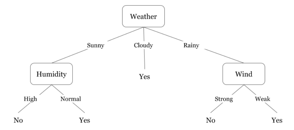
In machine learning, we use decision trees also to understand classification, segregation, and arrive at a numerical output or regression. The name itself suggests that it uses a flowchart like a tree structure to show the predictions that result from a series of feature-based splits. It starts with a root node and ends with a decision made by leaves.

In an automated process, we use a set of tools to do the actual process of decision making and branching based on the attributes of the data. The originally unsorted data, at least according to our needs, must be analyzed based on a variety of attributes in multiple steps and segregated to reach lower randomness or achieve lower entropy.

While completing this segregation, the algorithm needs to consider the probability of a repeat occurrence of an attribute. Therefore, we can also refer to the decision tree as a type of probability tree. The data at the root node is quite random, and the degree of randomness is called entropy. As we break down and sort the data, we arrive at a higher degree of accurately sorted data and different degrees of information.

Let’s get familiar with some of the terminologies about decision tree.

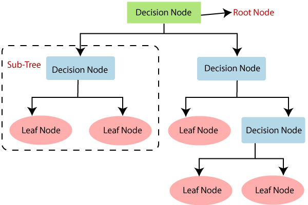
• Root Node:
  • This node gets divided into different homogeneous nodes. It represents the entire sample.
• Decision Nodes:
  • The nodes we get after splitting the root nodes are called Decision Node.
• Leaf Nodes:
  • The nodes where further splitting is not possible are called leaf nodes.
• Sub-tree:
  • Just like a small portion of a graph, a sub-section of this decision tree is called sub-tree.
• Pruning:
  • It is nothing but cutting down some nodes to stop overfitting.
• Splitting:
  • It is the process of splitting or dividing a node into two or more sub-nodes.
• Interior Nodes:
  • They represent different tests on an attribute.
• Branches:
  • They hold the outcomes of Interior Nodes’s tests.
• Parent and Child Nodes:
  • The node from which sub-nodes are created is called a parent node. And, the sub-nodes are called the child nodes.

To decide the feature split, different metrics are used to decide the best split in a top-down greedy manner i.e. the splitting begins from a state when all points belong to the same region and successive splits are made such that the resulting tree has a better metric value.
The following are commonly cost functions for different tasks:

• Entropy:
  • Measures the amount of uncertainty or randomness in the data. The objective is to minimize entropy in order to achieve homogeneous regions i.e. regions having data points belonging to a similar class.
• Gini index:
  • Measures the likelihood that a randomly selected data point would be misclassified by a particular node.
• Information Gain:
  • Measures the reduction in entropy/gini index that occurs due to a split. Tree-based algorithms either use Entropy or Gini index as a criteria to make the most informative split i.e. split that reduces the criteria by the most amount.
• Residual Sum of Squares:
  • Measures the sum of squared difference between the target class and the mean response of decision region for each data point in a region.

How does Decision Tree work?

Decision trees work on the principle as described in the following.

1. All training instances are assigned to the root of the node i.e. to a single predictor space.
2. For each feature in the data set, divide the predictor space into decision regions for each feature value.
3. Calculate the cost function for each split performed.
4. Identify the feature and the corresponding feature value which leads to the best split. This feature-feature value combination constitutes the splitting condition.
5. Partition all instances into decision regions based on the splitting condition.
6. For each decision region, continue this process until a stopping condition is reached.
7. Once the decision tree has been constructed, it can be used to evaluate new instance. The new instance is first placed in the corresponding decision region based on the tree logic and the aggregated measure of all the training target values is predicted for the instance.

How many splits?

As this splitting process is repeated, the tree keeps on growing and becomes more complex. At this point, the algorithm starts learning noise in the data set. This results in overfitting i.e. the model becomes too specific to a dataset that it is trained on and can not generalize well on other unseen data sets. In order to avoid this situation, a technique called pruning is incorporated.
Pruning aims at getting rid of sections of the tree that have low predictive power. It can be done by limiting the maximum depth of the tree or by limiting the minimum number of samples per region.

Improve the model

There are several ways to improve decision tree models, each one addressing a specific shortcoming of this machine learning algorithm.

• Minimum samples for leaf split:
  • Determine the minimum number of data points which need to be present at leaf nodes. If an additional split at a leaf node would cause two branches, where at least one branch would have less than the minimum sample of nodes, the leaf node cannot be split further. This prevents the tree from growing too close to samples.
• Maximum depth:
  • Setting maximum depth allows you to determine how deep a tree can get. Shallower trees will be less accurate but will generalize better, while deeper trees will be more accurate on the training set, but have generalization issues with new data.
• Pruning:
  • In pruning, an algorithm starts at the leaf nodes and removes those branches, which, after the removal, do not affect the overall tree accuracy on the test dataset. Effectively, this method preserves a high tree performance, while lowering the complexity of the model.
• Ensemble methods:
  • Ensemble methods combine multiple trees into an ensemble algorithm. The ensemble uses tree voting as a mechanism to determine the true answer. For classification problems, ensemble algorithms pick the mode of the most often predicted class. For regression problems, ensemble algorithms take the mean of the trees prediction. A special case of ensemble methods is the random forest, one of the most successful and widely used algorithms in machine learning.
• Feature selection:
  • To avoid overfitting on sparse data, either select a subset of features or reduce the dimensionality of your sparse dataset with appropriate algorithms e.g. PCA.

Advantages of Decision Tree

• Easy to understand. Since the decision regions are produced based on boolean relations, these methods can be graphically visualized to gather an intuitive understanding of what the algorithm does.
• Can handle nonlinear relationships between features and target.
• Can work with categorical and numerical data unlike regression models where categorical data needs to be one-hot encoded.
• Non-parametric: These methods do not make any assumption regarding distribution, independence, or constant variance of the underlying data that it processes. This is vital in applications where very little is known about the data and which features to use to make predictions.
• Unlike distance-based methods, these algorithms do not require feature scaling i.e. normalization or standardization of data before feeding to the model.

Disadvantages of Decision Tree

• Generally, have poor accuracy and are called weak learners.
• Prone to overfitting.
• A slight change in dataset can lead to a significant change in tree structure.

Most application of decision tree algorithm is Highly utilized in fields, where modeling and interpreting human behavior is the primary focus. These include marketing use cases and customer retention.

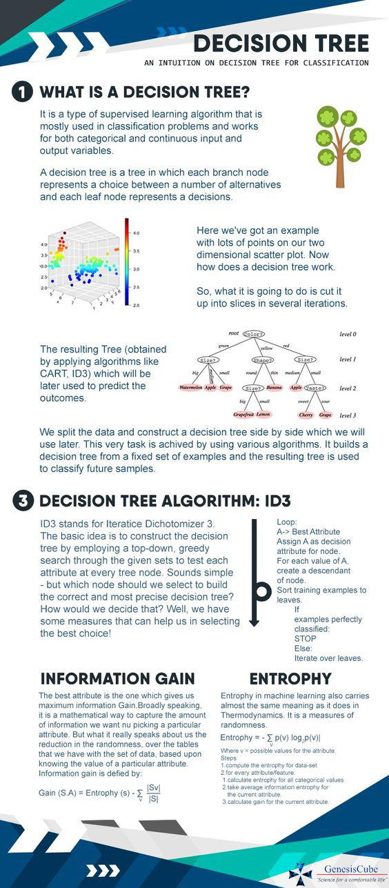
Infographic

Hope you found this post useful. Feel free to share your feedback.

Recommended for you:
Random Forest Algorithm explained
Hierarchical Clustering Python