GenesisCube

Ensemble Learning in Machine Learning

Machine learning predictions follow following behavior. Models process given inputs and produce an output. The output is a prediction based on what pattern the models see during the training process. But in many cases we need multiple models. here comes ensemble learning. Ensembling is the technique to combine several individual predictive models to come up with the final predictive model.
In this post, we’re going to look at the ensembling techniques.

Bagging Technique

Bagging is based on making the training data available to an iterative learning process. Each model learns the error produced by the previous model using a slightly different subset of the training dataset.
The idea behind bagging is combining the results of multiple models to get a generalized result. Here’s a question: If you create all the models on the same dataset and combine it, there is a high chance that these models will give the same result since they are getting the same input. One of the techniques to solve this problem is bootstrapping.
Bootstrapping is a sampling technique in which we create subsets of observations from the original dataset, with replacement. Bagging (or Bootstrap Aggregating) technique uses these subsets (bags) to get a fair idea of the distribution (complete dataset). The size of subsets created for bagging may be less than the original dataset.
Bagging reduces variance and minimizes overfitting. One example of bagging technique is the random forest algorithm.

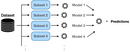
Bagging works in the below steps.

1. Multiple subsets are created from the original dataset, selecting observations with replacement.
2. A base model also known as a weak model is created on each of these subsets.
3. The models run independent and parallel on subsets.

Boosting Technique

This is an ensemble of algorithms, where we build models of several weak learners. In boosting technique, multiple weak-learners ( Those learners are called weak, because they are typically simple with limited prediction capabilities.) are learned sequentially. Each subsequent model is trained by giving more importance to the data points that were misclassified by the previous weak-learner. In this way, the weak-learners can focus on specific data points and can collectively reduce the bias of the prediction. The complete steps are shown in the diagram below.

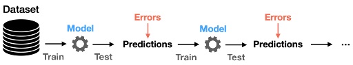
The first weak-learner is trained by giving equal weights to all the data points in the dataset. Once the first weak-learner is trained, the prediction error for each point is evaluated. Based on the error for each data point, the corresponding weight of the data point for the next learner is updated. If the data point was correctly classified by the trained weak-learner, its weight is reduced, otherwise, its weight is increased. Apart from updating the weights, each weak-learner also maintains a scalar alpha that quantifies how good was the weak-learner in classifying the entire training dataset.
The subsequent models are trained on these weighted sets of points. One way of carrying out training on a weighted set of points is to represent the weight term in the error. weighted mean squared error is used ensuring that data points with higher assigned weight, are given more importance in being correctly classified.
In the inference phase, the test input is fed to all the weak-learners and their output is recorded. The final prediction is achieved by scaling each weak-learner’s output with the corresponding weak-learner’s weight alpha before using them for voting.

There are lots of boosting algorithms but by far the best ones are Gradient Boosting and AdaBoost (Adaptive Boosting). The adaptation capability of AdaBoost made this technique one of the earliest successful binary classifiers.

Boosting works in the below steps

1. A subset is created from the original dataset.
2. Initially, all data points are given equal weights.
3. A base model is created on this subset.
4. This model is used to make predictions on the whole dataset.
5. Errors are calculated using the actual values and predicted values.
6. The observations which are incorrectly predicted, are given higher weights.
7. Another model (this tries to correct the errors from the previous model) is created and predictions are made on the dataset.
8. Similarly, multiple models are created, each correcting the errors of the previous model.
9. The final model or strong learner is the weighted mean of all the weak learners.

The boosting algorithm combines a number of weak learners to form a strong learner. The individual models would not perform well on the entire dataset, but they work well for some part of the dataset. Thus, each model actually boosts the performance of the ensemble.

Stacking Technique

Stacking is similar to bagging; they produce more robust predictors. In stacking, multiple weak-learners are trained in parallel, which is similar to what happens in bagging, but stacking does not carry out simple voting to aggregate the output of each weak-learner to calculate the final prediction. Rather, another meta-learner is trained on the outputs of weak-learners to learn a mapping from the weak-learners output to the final prediction. The complete steps are shown in the diagram below.

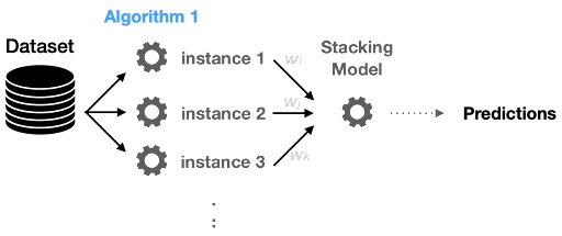
Stacking usually has weak-learners of different types. Hence a simple voting method that gives equal weights to all the weak-learners prediction doesn’t seem like a good idea (it would have been if the weak-learners were identical in structure). That is where the meta-learner comes in. It tries to learn which weak-learner is more important.
The weak-learners are trained in parallel, but the meta learner is trained sequentially. Once the weak-learners are trained, their weights are kept static to train the meta-learner. Usually, the meta-learner is trained on a different subset than what was used to train the weak-learners.

Stacking works in the below steps

1. The train dataset is split into 10 parts.
2. A base model (suppose a decision tree) is fitted on 9 parts and predictions are made for the 10th part. This is done for each part of the train dataset.
3. The base model is then fitted on the whole train dataset.
4. Using this model, predictions are made on the test set.
5. Steps 2 to 4 are repeated for another base model resulting in another dataset of predictions for the train dataset and test dataset.
6. The predictions from the train dataset are used as features to build a new model.
7. This model is used to make final predictions on the test prediction dataset.

Blending Technique

Blending is similar to the stacking approach, except uses only a holdout validation dataset from the train dataset to make predictions. In other words, the predictions are made on the holdout dataset only. The holdout dataset and the predictions are used to build a model which is run on the test dataset.

blending works in the below steps

1. The train dataset is split into training and validation datasets.
2. Models are fitted on the training dataset.
3. The predictions are made on the validation datasetand the test dataset.
4. The validation dataset and its predictions are used as features to build a new model.
5. This model is used to make final predictions on the test and meta-features.

Recommended for you:
Random Forest Algorithm explained
Genetic Algorithm in Machine Learning