GenesisCube

Gradient Boosting Algorithm Explained

While learning about the Machine Learning models, you might have heard a lot about Boosting. In this post, we will discuss one of the most trending algorithms that we use for prediction in Machine Learning.

What is Gradient Boosting?

It is more commonly known as the Gradient Boosting Machine. It is one of the most widely used ensembling techniques when we develop predictive models.
The aim of the algorithm lies in developing a first-hand model structure based on the training dataset. Then, we develop the second model to resolve the drawbacks of the previous model. Let us try to understand this definition.

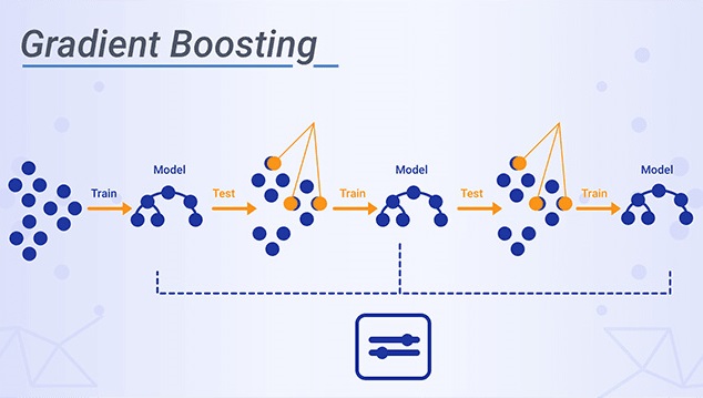
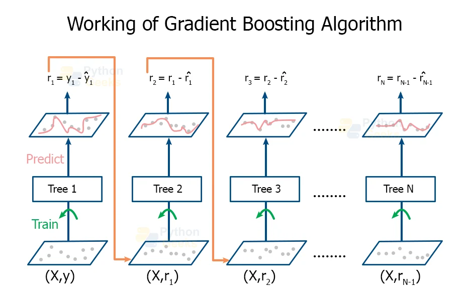
The algorithm focuses upon developing a sequential structure of models that try to reduce the errors by rectifying the results of the residuals of the previous models.
Gradient boosting creates an ensemble of trees, this technique is called boosting because we expect an ensemble to work much better than a single estimator.

The type of algorithm that we use depends on the type of problem we need to tackle. We deploy the Gradient Boosting Regressor when we have to deal with a continuous values and the Gradient Boosting Classifier when we have to use it for discrete values.
Difference between these two problems is the use of “loss function”. The main focus of the algorithm is to minimize the loss function in order by repetitively adding weak learners.

It tends to train many models in a gradual, additive, and sequential.
The Gradient Boosting model explores the shortcomings by making use of gradients in the loss function (y = ax+b+e, e needs a special mention as it is the error term).
Loss function accounts to be a measure indicating how good are model’s coefficients are at performing fitting the underlying data.

Gradient Boosting Hyperparameters

Hyperparameters are key parts of algorithms which effect the performance and accuracy of the model. Learning rate and n_estimators are two critical hyperparameters of gradient boosting.

• Learning Rate
  • denoted as ‘α,’ controls how fast the model learns. This is done by multiplying the error in previous model with the learning rate and then use that in the subsequent trees.
  • The lower the learning rate, the slower the model learns. Each added tree modifies the overall model.
  • The advantage of slower learning rate is that the model becomes more robust and efficient and avoids overfitting. However, learning slowly comes at a time-cost. It takes more time to train.
• n_estimator
  • is the number of trees used in the model. If the learning rate is low, we need more trees to train the model. However, we need to be careful at selecting the number of trees. too many trees create a high risk of overfitting.

Gradient Boosting Mathematics

Let’s discuss maths behind the algorithm step-by-step.
The output model y when fit to only 1 decision tree, is given by:

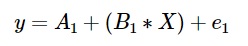
Where, e_1 is the residual from this decision tree.
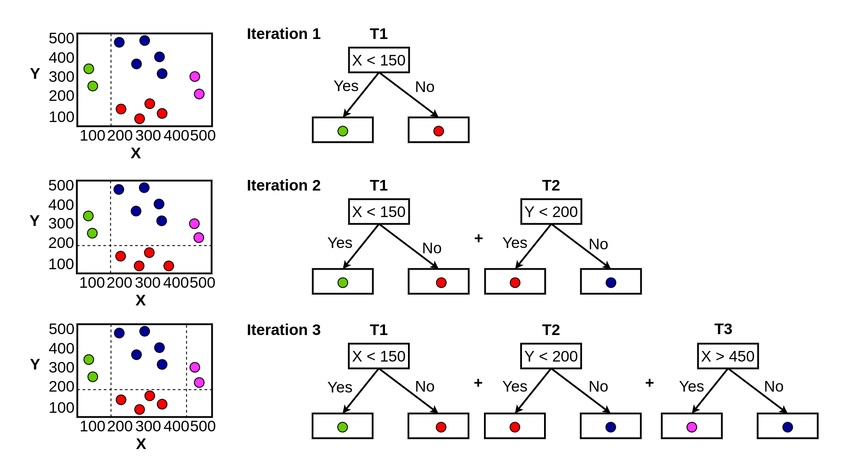
We fit the consecutive decision trees on the residual from the last one. So when gradient boosting is applied to this model, the consecutive decision trees will be mathematically represented as:

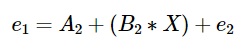
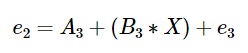
In an actual model, number of learners or decision trees is much more. Final model of the decision tree will be given by:

Gradient Boosting Working

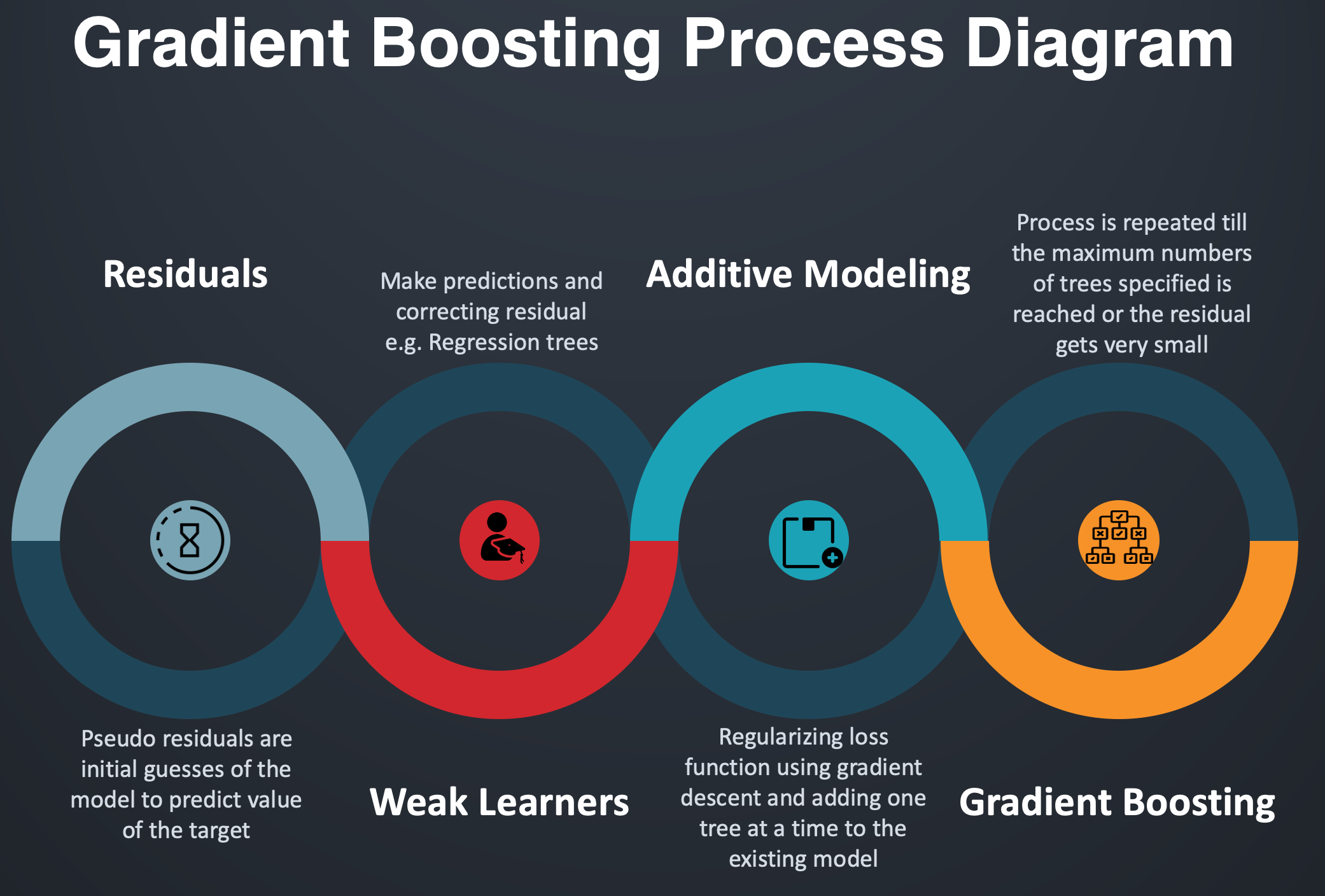
Working of Algorithm can be divided on the basis of major three elements:

• Optimizing the Loss Function.
  • There are many functions available for usage, but the loss function that we use for the models, depends on the type of algorithm that we are using. The main focus of selecting any loss function is that the loss function should be differentiable.
  • The most beneficial feature of using this algorithm is that we do not need to derive a new boosting algorithm for each loss function that we use while solving the problem.
• Fabricating a weak learner.
  • While using algorithm we use decision trees as weak learners, whose outputs are real values for splits and we can add the outputs together, to allow subsequent models to add their outputs with the correct residual in the predictions.
  • Also, we construct these trees using the greedy algorithm by choosing the best split points that are based on the purity scores like gini or those who can minimize the loss function.
• Development of an additive model of weak learners to minimize the loss function.
  • We add the new trees one at a time in the model such that the pre-existing trees remain unaltered. We follow the gradient descent procedure in order to minimize the loss while adding the trees.
  • After the calculation of the loss, we modify the weights to minimize the error.

Gradient Boosting Infographic

We are always open to your questions and suggestions.
You can share this post on LinkedIn, Facebook, Twitter, so someone in need might stumble upon this.

Recommended for you:
Adaptive Boosting Algorithm Explained
XGBoost Algorithm Explained